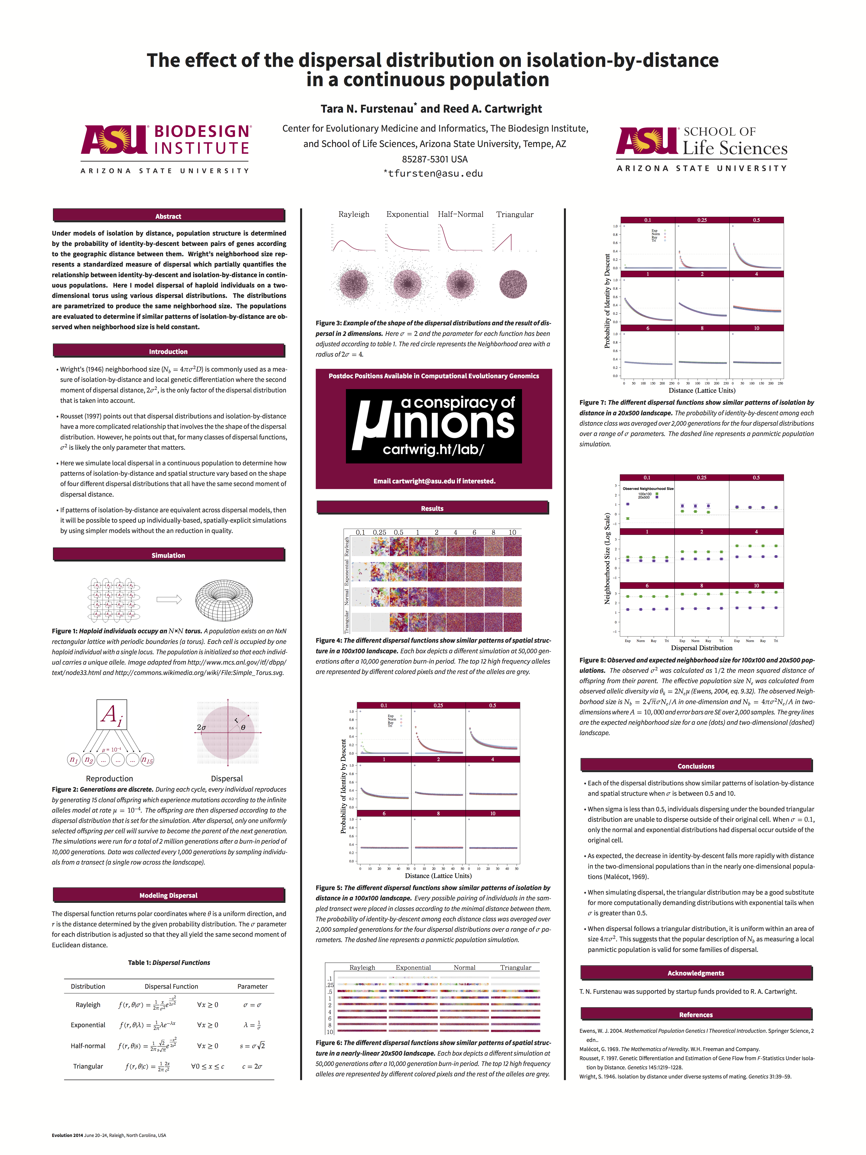
The effect of the dispersal kernel on isolation-by-distance in a continuous population

Tara N. Furstenau and Reed A. Cartwright

Abstract

Under models of isolation-by-distance, population structure is determined by the probability of identity-by-descent between pairs of genes according to the geographic distance between them. Well established analytical results indicate that the relationship between geographical and genetic distance depends mostly on the neighborhood size of the population, $N_b=4\pi\sigma^2D_e$ , which represents a standardized measure of dispersal. To test this prediction, we model local dispersal of haploid individuals on a two-dimensional torus using four dispersal kernels: Rayleigh, exponential, half-normal and triangular. When neighborhood size is held constant, the distributions produce similar patterns of isolation-by-distance, confirming predictions. Considering this, we propose that the triangular distribution is the appropriate null distribution for isolation-by-distance studies. Under the triangular distribution, dispersal is uniform within an area of 4πσ2 (i.e. the neighborhood area), which suggests that the common description of neighborhood size as a measure of a local panmictic population is valid for popular families of dispersal distributions. We further show how to draw from the triangular distribution efficiently and argue that it should be utilized in other studies in which computational efficiency is important

PeerJ (Peer Reviewed Article)
arXiv
github

Evolution 2014 Poster

Simulation Description

In the simulation, a population exists on a $N \times N$ rectangular lattice with either periodic boundaries (a torus) or absorbing boundaries. Individuals are uniformly distributed on the lattice with a single individual per node. Individuals are haploid and contain a single, selectively neutral genetic locus.

In the initial generation, the population contains the maximum number of individuals allowed by the landscape and each individual is assigned a unique allele (represented by an integer). During each discrete generation cycle, individuals reproduce by producing a number of clonal offspring. These offspring experience mutations according to the infinite alleles model at rate $\mu$ . A burn-in period may be set to allow the population to reach a drift/mutation equilibrium.

The offspring disperse from their original cell according to a set dispersal distribution. As offspring land on their destination cell they are immediately accepted or rejected using a reservoir sampling method, which allows the offspring to be uniformly sampled at each location as they arrive instead of storing them all in memory (Vitter, 1985). When dispersal is complete, there is a maximum of one offspring per cell and that offspring becomes a parent in the next generation.

There are currently 9 different dispersal distributions: exponential, gamma, half-normal, Pareto, Rayleigh, Rice, ring, and uniform. Some distributions have two implementations where one version is faster than the other. The faster version is used by setting the --fast flag to true which is default. All uniform pseudo-random numbers are generated using an efficient xorshift algorithm (Marsaglia 2003).

Exponential

The exponential dispersal function takes a single argument ( $\sigma$ ) and returns polar coordinates with exponentially distributed distances with rate $\frac{1}{\sigma}$ and a uniform angle. The distance values are drawn using an implementation of the ziggurat rejection sampling algorithm for the exponential distribution (Marsaglia and Tsang, 2000).

Gamma

The gamma dispersal function takes two arguments, $\sigma$ and $\alpha$ , and the $\beta$ parameter is calculated so that the second moment of the distribution is equal to $2\sigma^2$ . This function returns polar coordinates with gamma distributed distances and a uniform angle. The distance values are generated using Marsaglia’s (2000) rejection sampling algorithm which takes advantage of the fast ziggurat procedure for generating normally distributed PRNs (Marsaglia and Tsang, 2000).

Half-Normal

The half-normal dispersal function takes a single argument, $\sigma$ , and returns polar coordinates with half-normal distributed distances with variance parameter $\sigma\sqrt{2}$ and a uniform angle. The distance values are the absolute value of draws from a normal distribution using an implementation of the ziggurat rejection sampling algorithm (Marsaglia and Tsang, 2000).

Pareto

The Pareto distribution is a mixture of exponential distributions with a gamma mixing distribution. The Pareto dispersal function takes two arguments, $\sigma$ and $\alpha$ and the $X_{min}$ parameter is calculated so that the second moment of the distribution is equal to $2\sigma^2$ . The function returns polar coordinates with Pareto distributed distances and a uniform angle. The distance values are generated using inverse transform sampling, which, due to the relationship between the Pareto and exponential distributions, takes advantage of the fast ziggurat procedure for generating exponentially distributed PRNs (Marsaglia and Tsang, 2000).

Lomax

The Lomax distribution or Pareto Type II distribution is essentially a Pareto distribution that has been shifted so that its support begins at zero. It takes two arguments, $\sigma$ and $\alpha$ and the scale parameter is calculated so that the second moment of the distribution is equal to $2\sigma^2$ . The function returns polar coordinates with Lomax distributed distances and a uniform angle. The distances are generated by subtracting Xmin from the Pareto dispersal function.

Rayleigh

The Rayleigh dispersal function may take one or two arguments, $\sigma_x$ and $\sigma_y$ . If only a single argument is given, $\sigma$ will be the same for each dimension and result in an isometric 2-dimensional normal distribution. For the sake of uniformity, this was called the Rayleigh dispersal function because it originally returned polar coordinates with Rayleigh distributed distances and a uniform angle; however, this required an inefficient conversion from polar to Cartesian coordinates. We instead draw axial offset distances from a normal distribution with variance $\sigma_x^2$ (or $\sigma_y^2$ ) using an implementation of the ziggurat rejection sampling algorithm (Marsaglia and Tsang, 2000). There is a “fast” version of this dispersal function available which precalculates the probability of dispersing on a discrete lattice. Once the dispersal probabilities are calculated we use the efficient Alias method to sample from this discrete probability distribution (Vose, 1991).

Rice

The Rice dispersal function takes two arguments, $\sigma$ and $angle$ . This distribution results in an isometric 2-dimensional normal distribution where the mean has shifted away from the origin to a polar coordinate ( $v,angle$ ). The $v$ parameter is calculated so that the second moment of the distribution is equal to $2\sigma^2$ . Axial distances are drawn from two normal distributions with means $v\cos(angle)$ and $v\sin(angle)$ and variance $\sigma^2$ using an implementation of the ziggurat rejection sampling algorithm (Marsaglia and Tsang,2000).

Ring

The ring dispersal function takes two arguments, $\sigma$ and $p$ . This distribution returns a polar coordinates with a constant distance $\sigma$ and a uniform angle. The $p$ parameter determines the probability of not dispersing away from the origin. There is a fast version of this dispersal function available which precalcuates the probability of dispersing on a discrete lattice. Once the dispersal probabilities are calculated we use the efficient Alias method to sample from this discrete probability distribution (Vose, 1991)

Triangular

The triangular dispersal function takes a single argument, $\sigma$ , and returns polar coordinates with triangular distributed distance with $a=0$ , $b=c=2\sigma$ , and a uniform angle. The distance values are generated using inverse transform sampling. There is a fast version of this dispersal function available which precalcuates the probability of dispersing on a discrete lattice. Once the dispersal probabilities are calculated we use the efficient Alias method to sample from this discrete probability distribution (Vose, 1991).

Uniform

The uniform dispersal function takes two arguments, the $x$ and $y$ dimensions of the landscape. It returns new coordinates anywhere on the landscape with uniform probability.

Compiling from Source Code

IBD requires CMake 2.8 to build from source.

Download the source code.
Decompress the tar-bzip archive
```
  tar xvzf IBD-*.tar.bz2
```
Change to the build directory.
```
  cd IBD-*/build
```
Run the CMake build system.
```
  cmake ..
```
Compile
```
  make
```

Dependencies

The Boost c++ Library is required for compilation and usage.

Foreach
Program Options

Run

Usage:

$ ./ibd config.txt
$ ./ibd --help
Allowed Options:

General Options:
  --help                Produce help message

Configuration:
  -x [ --maxX ] arg (=100)              Set X dimension
  -y [ --maxY ] arg (=100)              Set Y dimension
  -g [ --generations ] arg (=10)        Set number of Generations to run after
                                        burn-in
  -o [ --offspring ] arg (=10)          Set number of offspring per individual
  -m [ --mut ] arg (=0)                 Set mutation rate
  -d [ --distribution ] arg (=triangular)
                                        Set Dispersal Distribution
  -s [ --sigma ] arg (=2)               Set dispersal parameter
  -b [ --burn ] arg (=0)                Set Burn-in Period
  -t [ --sample ] arg (=1)              Sample every n generations after
                                        burn-in
  -f [ --output_file ] arg (=data)      Output File Name
  --seed arg (=0)                       Set PRNG seed, 0 to create random seed
  --landscape arg (=torus)              Set boundary conditions: torus or
                                        rectangular
  --transect arg (=0)                   Set position of transect in X axis.
  --verbose arg (=0)                    Print data to screen
  --sparam arg (=0)                     Extra Parameter for dispersal
  --fast arg (=1)                       Use fast dispersal when available